Calculating RMS Acceleration from a PSD Breakpoint Table in Random Vibration Testing

In the V&V field of automotive components, random vibration testing is an essential process. Typically, V&V engineers select a specific PSD breakpoint table and Power Spectral Density (PSD) plot from the ISO 16750-3 standard based on the installation position of the product in the vehicle, and then proceed with the test. Therefore, many might not have considered how to directly calculate the RMS acceleration value from the PSD breakpoint table.

However, I encountered a unique situation in a recent project. For one of the products in this project, our company required the random vibration test to have an RMS acceleration value of no less than 6g, equivalent to 58.8 m/s². However, according to the ISO 16750-3:2023 standard, the PSD breakpoint table in section 4.1.9 corresponds to an RMS acceleration value of 57.9 m/s², slightly below 6g. While the PSD breakpoint table in section 4.1.5 corresponds to an RMS acceleration value of 68.7 m/s², which meets our requirements, the supplier was reluctant to adopt this solution due to the higher associated risk. Therefore, they proposed adjusting the PSD breakpoint table in section 4.1.9 to achieve an RMS acceleration value slightly above 6g.

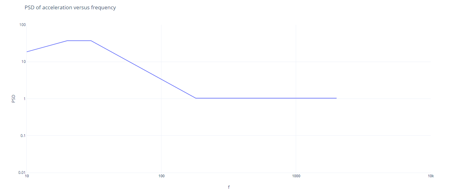
Following this idea, they contacted the vibration shaker supplier, who used the software on the shaker to slightly adjust the PSD breakpoint table from section 4.1.9. They then informed me that the adjusted PSD breakpoint table corresponds to an RMS acceleration value of 59.29 m/s². The adjusted PSD breakpoint table and PSD plot are shown below.

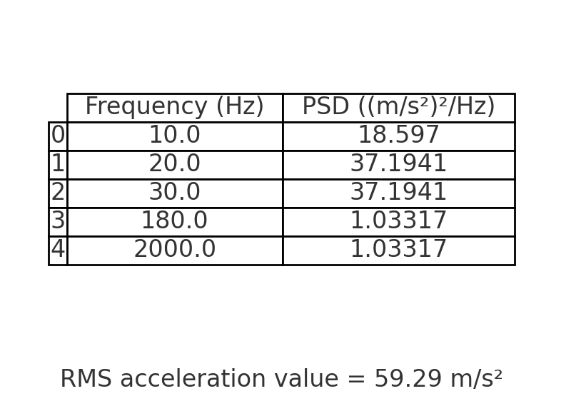
At that time, I wanted to calculate the RMS acceleration value myself based on the adjusted PSD breakpoint table to verify whether the result of 59.29 m/s² was accurate.

My initial thought process was very simple: observe the units. The unit of PSD on the vertical axis is (m/s²)²/Hz, and the unit of frequency on the horizontal axis is Hz. The product of these two units is (m/s²)², and the product of the values on the horizontal and vertical axes corresponds to the area under the PSD curve on the PSD plot. Looking at the PSD plot, the area under the PSD curve is very regular, either rectangles or trapezoids. If I calculate the sum of these areas and then take the square root, I should get the RMS acceleration value I need. It didn’t seem like a complicated task. However, when I calculated it, I was shocked—the result I got was 73.47 m/s², which was significantly different from the 59.29 m/s² calculated by the vibration shaker software.

Later, I consulted with a Ph.D. colleague in my company, and his thought process was consistent with mine, so he also couldn’t figure out where the problem was.

At that time, due to a busy schedule, I couldn’t delve deeper into the issue and chose to trust the vibration shaker software’s calculation results, incorporating this value into the test specification. After all, they only made slight adjustments to the PSD breakpoint table in section 4.1.9 of the ISO 16750-3:2023 standard, so it seemed reasonable that the calculated result would be close to the value in the standard.

Then I had almost forgotten about this matter, but as the project progressed into DV and PV phases, I unexpectedly discovered that different vibration shakers produced slightly different target RMS acceleration values even when using the same PSD breakpoint table. For example, during DV testing, the vibration shaker yielded a target RMS acceleration value of 59.29 m/s², while during PV testing, the vibration shaker only produced a target RMS acceleration value of 58.94 m/s², slightly lower than the DV RMS acceleration target. This raised a critical question: should the PV test result be accepted?

To resolve this issue, I decided to thoroughly understand how to derive and calculate the corresponding RMS acceleration value based on the PSD breakpoint table, and to find out where my original calculation method went wrong.

After some observation, I finally realized the root of the problem. The PSD plot uses logarithmic scales on both the horizontal and vertical axes. The straight lines that appear in this logarithmic coordinate system are not straight lines in a linear coordinate system, and therefore, the area they cover in a linear coordinate system is not a simple trapezoid.

Once I realized this, the process became clear. Below, I have outlined the detailed calculation steps, for reference.

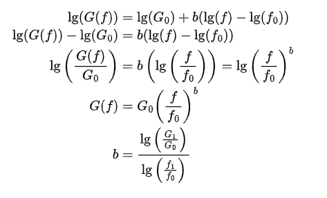
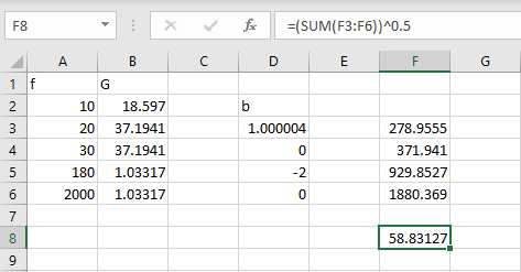
Suppose there is a straight line on the PSD plot, with the leftmost point being (f0, G0) and the rightmost point being (f1, G1). The coordinates of any point on this line between these two points can be expressed as (f, G(f)). According to analytic geometry, the initial and final simplified forms of the equation for this line are shown below, where b represents the slope of the line in the logarithmic coordinate system.

With the expression for G(f) and the formula for calculating b, we can use the principle of integration to calculate the RMS acceleration value.

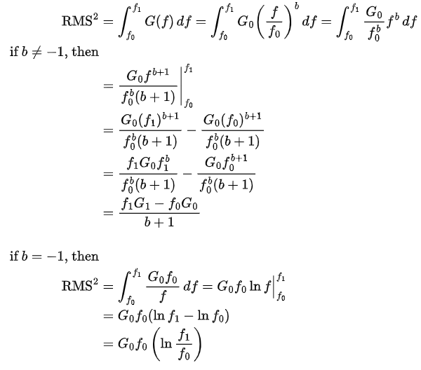
Based on the formulas above, we can calculate the b values and RMS square values for each line segment on the PSD plot. Summing the RMS square values for each segment and then taking the square root yields the final result. To simplify the process, I entered the formulas into an Excel spreadsheet and ultimately obtained an RMS acceleration value of 58.83 m/s². This should be the correct RMS acceleration value corresponding to the slightly adjusted PSD breakpoint table. Since the target RMS acceleration value of 58.94 m/s² obtained during the PV test is slightly higher than this calculated value, it can be considered an acceptable result.

After reviewing the current PSD plots in the ISO 16750-3 standard, it appears that they are still primarily composed of various straight lines. This indicates that the calculation method I described above has broad applicability in the current V&V random vibration testing. I hope this information can be beneficial in your daily work. If you have any questions, please leave them in the comments.